

VITICULTURE / Original research article
Abstract
Facing the challenges posed by climate change, quantifying the resilience of wine terroirs is imperative. Total Transpirable Soil Water (TTSW) represents the maximum water volume that vines can extract from soil, a critical parameter for water balance models. Current TTSW estimation methods often require expensive protocols, limiting their use in commercial vineyards and over large regions. This research aimed to evaluate a low-cost TTSW estimation method that combines Inverse Modelling (IM) with crowdsourced data. The chosen IM method, which has been validated locally, relies on observations of vine shoot growth (iG-Apex), weather data and satellite images. More precisely, the IM relies on a process-based relationship linking the decline in plant water status expressed as a slope coefficient, primarily inferred from plant growth and weather data, to the transpiration rate under bare soil and dry conditions, that is based on the basal crop coefficient (Kcb). By integrating a crowdsourced database, the IM method estimates TTSW at numerous locations where data were collected. A case study was carried out in a Southern French wine appellation (“Côtes du Rhône”), and a TTSW map defined by local experts was used for qualitative evaluation. The method produced TTSW estimates between 60 and 190 mm. High-confidence areas, where expert opinions converged and at least four field-level TTSW estimates existed, demonstrated coherent TTSW rankings. Two distinct geographical regions were identified: one characterised by low-to-medium TTSW and another by medium-to-high levels. This spatial differentiation suggests that crowdsourced data, when combined with inverse modelling, can effectively reveal broad-scale TTSW patterns. However, inaccurate estimates persisted in some areas. A large proportion of crowdsourced observations were excluded from the inversion due to insufficient time series length. This work demonstrates the capacity of farmer-generated plant observations to quantify the spatial patterns of a critical agronomic variable at the regional scale. The case study illustrates how farmers and viticulture professionals can contribute, through crowdsourcing, to the collective quantification of TTSW, a key variable for developing coordinated adaptation strategies in Mediterranean viticulture under climate change.
Introduction
Climate change is affecting water availability for vineyards globally (Santillán et al., 2019). In some important commercial winegrowing estates where dry-farming systems are predominant, vines are increasingly affected by the negative effects caused by irregular rainfall patterns or droughts. Therefore, it is essential to quantitatively assess vineyards’ vulnerabilities under changing environmental conditions (van Leeuwen et al., 2018). One critical indicator that quantitatively evaluates the resilience against droughts is the Total Transpirable Soil Water (TTSW), which represents the maximum volume of water that vines can extract from the soil; it corresponds to the difference between field capacity and permanent wilting point, below which the plant can no longer generate sufficient suction to withdraw water from soil pores (Pellegrino et al., 2005). TTSW is a crucial parameter in soil water balance models (Celette et al., 2010), enabling the estimation of water available for plants, therefore supporting decision-making processes related to vine canopy and/or cover crop management and/or to irrigation.
Understanding the spatial TTSW variation is crucial (Brillante et al., 2015), as this knowledge is tightly linked to farming practices which maintain a wine’s "terroir expression”. Indeed, the dynamic of vine water status over a season plays a key role in yield elaboration and berry metabolism (Menn et al., 2020). Spatial knowledge of TTSW enables the implementation of site-specific management practices that address heterogeneous vine water status dynamics within a wine appellation, thereby supporting the preservation of a consistent wine quality.
Nonetheless, precisely measuring TTSW for vines poses significant challenges due to operational constraints (Coppola et al., 2013). Being a perennial crop, vine TTSW is hard to measure because its roots can be both deep and unevenly distributed (Pellegrino et al., 2005). Hence, localised assessments of TTSW require substantial investment, which makes the spatial mapping of TTSW highly difficult. Some authors have tried to study the TTSW variation at a field scale (Acevedo-Opazo et al., 2008), while few studies have been conducted at regional or within-region scales (Fernandez-Mena et al., 2023).
Leenaars et al. (2018) proposed a Digital Soil Mapping approach to obtain spatial estimates of TTSW. Those authors estimated both the soil water holding capacity and the soil depth explored by maize (i.e., rootability) for accounting for soil–plant interactions, a key aspect to quantify TTSW. However, the implementation of their approach could be complicated for wine grapes, because the rootability for the perennial crop might be difficult to characterise (Lakso & Eissenstat, 2012). On the contrary, Coulouma et al. (2020) proposed a spatial TTSW estimation method specifically for vineyards based on berries’ carbon isotope discrimination by the time of harvest, which reveals the cumulative water deficit suffered by vines during berry maturation. The interest of this information is that it can be obtained at many locations with less restrictive logistical constraints. Nonetheless, this approach did not make direct quantification of TTSW, rendering it difficult to integrate the results in water balance models or other decision support tools. Additionally, at a large spatial scale, the sampling and analysis could be costly.
Comparatively, Inverse Modelling (IM) is a cost-efficient approach which is increasingly adopted for retrieving TTSW (Cousin et al., 2022). The IM approach is applied when the targeted variable, like TTSW, is an input of a process-based model, and when obtaining that model’s output data is easier than obtaining the variable itself (Zhang et al., 2024a). Thanks to the emergence of new data sources with a high spatial coverage rate, retrieving vines’ TTSW at extended spatial scales is becoming possible. Alkassem et al. (2022) proposed a TTSW retrieval method for vineyards by using satellite-image-based Leaf Area Index, evapotranspiration, and in-situ soil moisture measurements (depth of 0.2–0.3 m). Although the results were promising, obtaining these data sources can be logistically constraining for small vineyard owners, especially when multiple locations must be handled, which limits the applicability of this approach for estimating TTSW in a production context.
Zhang et al. (2025) introduced an inversion method tailored for Mediterranean rainfed vineyards. This method deployed simple observations of vine shoot growth, an indicator of vine water status (Pichon et al., 2023), named iG-Apex, to provide a low-cost way for estimating TTSW. Complementing this, a freely available mobile application, Apex-Vigne (Brunel et al., 2019), has been facilitating the collection of iG-Apex by viticultural professionals, creating a crowdsourced database at a regional scale (Pichon et al., 2022). In 2023, this initiative has gathered over 30,000 observations of iG-Apex, primarily from Southern France where the Mediterranean climate emphasises the need to monitor vine water status during summers.
This database, stemming from crowdsourcing, could be a promising data source to be coupled with the Inverse Modelling approach of Zhang et al. (2025). Nevertheless, crowdsourced data have many limitations. First, such data is collected from a wide range of vineyards with diverse training systems and cultivars: part of the variability in iG-Apex data may therefore be caused by these factors and not by TTSW. Additionally, the sampling is opportunistic, and data collectors are free to choose the locations and timing for measurements, leading to spatially heterogeneous, heterotopic, and temporally asynchronous data (Pichon et al., 2021). Other factors may also influence iG-Apex data, like the operator effect (Pichon et al., 2023) or farming practices (e.g., weeding and cover crop management). Overall, crowdsourced observations are often uncertain, and this uncertainty propagates to any variables estimated from them. However, despite these sources of uncertainty, the large amount of data generated by crowdsourcing may provide information that is rich enough for offsetting the low quality of individual pieces of data (i.e., "the wisdom of crowds"; Surowiecki, 2004).
In this context, this paper explored the potential of a five-year (2019–2023) crowdsourced database that contained vine shoot growth observations for retrieving TTSW through the approach of Inverse Modelling. The study focused on a wine appellation in the French Mediterranean basin: Côtes du Rhône, which extends over 1200 km2. Due to the lack of ground-truth data of TTSW at this spatial scale, a focus group with local experts was convened to qualitatively evaluate the TTSW estimates.
Materials and methods
1. General description of crowdsourced data
The crowdsourcing tool was a free smartphone application called Apex-Vigne (Brunel et al., 2019). It allowed users to generate the index of vine shoot growth, known as iG-Apex, by observing fifty vine shoots from approximately ten mature, non-senescing vines (Vitis vinifera L.). Users were required to categorise these shoots into three growth stages: i) full growth, ii) moderate growth, and iii) stopped growth, which were weighted by different values: 1, 0.5, and 0, respectively (Pichon et al., 2023). The iG-Apex was then calculated as an average of the weights of the observed vine shoots, ranging on a continuous scale from 1 (full shoot growth) to 0 (total cessation of growth). Hence, lower values were taken to reflect a higher level of water deficit experienced by the measured vines.
Hundreds of growers and advisors have been using the Apex-Vigne application as an easy tool for estimating vine water status in the field. By making observations of vine shoot growth, they generated iG-Apex measurements. Measurements were georeferenced and transmitted to a database via the users’ smartphone internet connection. The mobile application also collected other meta-information, such as date of measurement, user’s identity and identity of the plot where the observation was collected. In this study, time series (TS) were defined as groups of iG-Apex measurements that shared the same plot identity and were carried out in the same year.
2. Retrieving TTSW with an inverse model
2.1. Presentation of the inverse model
Based on Gaudin et al. (2017), Zhang et al. (2025) proposed an adapted version of the inverse model to retrieve total transpirable soil water (TTSW) by using iG-Apex time series. To avoid repeating already developed methodologies, details regarding the inverse model are provided in Supplementary Information (SI).
The inverse model was validated at a local scale using experimental data, while manifesting an acceptable level of retrieval accuracy. The inverse model requires four inputs and can be presented by Equation 1:
(Equation 1)
where Kcb corresponded to the basal crop coefficient (no unit). It was assumed to represent the light interception capacity of vines at the flowering stage, and to be a constant number. The higher the Kcb value, the greater the potential water loss from the soil via transpiration (see SI 1.2).
The water status slope was fitted from a series of predawn leaf water potential (Ψpd, in MPa) values versus cumulative reference evapo-transpiration (ET0, in mm) recorded at the same dates (Gaudin et al., 2017). It quantified the rate at which soil water is depleted under a dry climatic condition, expressed in MPa/mm. A lower slope coefficient indicates that the soil dries out more quickly, as that signifies a sharper decrease in leaf water potential given the same amount of ET0 (see SI 1.2). Zhang et al. (2025) proposed to predict Ψpd from iG-Apex data collected under controlled field conditions. In this study, crowdsourced iG-Apex observations were used accordingly (see Section 2.2).
The plot area ratio is a formula specifically designed for integrating iG-Apex data, because this data can only be obtained at a plot (a group of ten adjacent productive vines) level. In a real field and notably in Mediterranean regions, a plot could often contain dead or missing vines (DMV) (Vaudour et al., 2017), which will increase the plot’s area. Therefore, this ratio aims to adjust the TTSW estimate given such variation of area, by dividing the area (in m²) of a referential measurement plot (which does not contain DMV) by the area of the actual plot (which may contain DMV) (Zhang et al., 2025). This ratio usually decreases the TTSW estimate with the presence of DMV.
The was a coefficient created during the development of the original inverse model (Gaudin et al., 2017). It does not have a direct physical meaning by itself, however, depends on the mathematical relationship between Ψpd and Fraction of Transpirable Soil Water (FTSW, a ratio between 0: no available soil water and 1: fully available soil water), according to the prior research of Lebon et al. (2003). It is assumed to be a constant value for rainfed vineyards (see SI 1.2).
Equation 1 was applicable under three specific conditions: (1) the considered period must be under dry conditions (i.e., no precipitation and irrigation); (2) water deficit level must be high enough for the vines to activate stomatal regulation; and (3) there is no capillary rise. In short terms, the method required a dry period where vines were suffering water deficit.
2.2. Inverse model inputs
Four data sources were used to obtain the inverse model inputs (Figure 1) required by the approach of Zhang et al. (2025). Certain inputs were associated with uncertainties, expressed as standard deviations (SD). The R package “errors” (Ucar & Henry, 2023) was used to propagate uncertainties of inverse model inputs towards TTSW estimates in each location where data were collected.
The Kcb was estimated from Sentinel-2 images using the regression model as proposed by Campos et al. (2010) that links Normalized Difference Vegetation Index (NDVI) and Kcb (“M1” in Figure 1). Extraction and pre-processing of Sentinel-2 images were performed with Google Earth Engine Code Editor. Pixels that overlapped with Crowdsourcing plots’ coordinates were extracted. When a plot did not have available satellite images, or too few (n < 10), a common value of 0.45 for Kcb was used (Rallo et al., 2021). The SD of Kcb was obtained from multiple Sentinel-2 images included in a time window that is suitable for making inversion. The length of each time window is specific to both year and location, because they are identified by checking local weather records so that the first inversion condition could be satisfied (Section 2.1). Therefore, those windows are generally positioned during the driest periods in summer. When the number of images was inferior to 10, a bibliographical SD value of 0.05 (Rallo et al., 2021) was considered.
The water status slope coefficients were obtained from Ψpd predictions and reference evapo-transpiration (ET0). A predictive model, named Recursive-Duo-Model (“M2” in Figure 1; Zhang et al., (2024b)), was used to derive Ψpd predictions from crowdsourced iG-Apex and weather data. The M2 required time series of iG-Apex containing at least three observations. It was trained using the complete dataset reported by Zhang et al. (2024b), originating from two Mediterranean rainfed vineyards and two red cultivars: cv. Syrah and cv. Grenache. Weather data were provided by Météo France (Bertuzzi & Clastre, 2022). Six weather variables were obtained at the daily scale and with an 8-km spatial resolution: ET0, mean, maximum and minimum temperature, precipitation, and relative humidity. Each TS was associated with weather data originating from the closest weather cell. The SD of water status slope was obtained by repeatedly running the Recursive-Duo-Model (n = 100) as proposed by Zhang et al. (2025).

Figure 1. Data sources used to feed inputs of the inverse model and retrieve total transpirable soil water (TTSW).
The plot area ratio was assumed to be 0.85, after consulting the specification document of the studied wine appellation (INAO, 2024), where the tolerance rate of dead or missing vines (DMV) was indicated. This setting was based on the hypothesis that each measurement plot was 15 % larger than a reference plot that contains no DMV. The SD of the plot area ratio was assumed to be 0.05 based on empirical knowledge.
In previous works, the value of was set to be 0.44 (Gaudin et al., 2017). To associate this quantity with uncertainty, the coefficient was re-estimated by combining the experimental data collected by Lebon et al. (2003) and Pellegrino et al. (2005). This consisted of repeatedly (2000 times) taking a random 60 % of the combined dataset and fitting the exponential model with the selected data (“Bootstrapping” in Figure 1). This allowed us to obtain an average and an SD of the coefficient from the 2000 sfitted models.
3. Crowdsourced data pre-processing
Due to the nature of crowdsourcing, raw collected data were pre-processed and enriched. The aim of enrichment was to increase the percentage of deployable data for making inversion. Before the enrichment, a quality filter was applied to all individual iG-Apex measurements to eliminate the invalid observations: duplicated measurements, those recorded outside of the vegetative period of the vine for the subsequent year (i.e., between October and April in the Northern Hemisphere).
3.1. Data enrichment
According to the specific conditions of the inverse model (Section 2.1), the inversion process had to be carried out during a dry period, where a minimum number (n = 3) of iG-Apex observations must be available. Depending on when and where observations were crowdsourced, it may happen that there were not enough observations in an iG-Apex time series (TS) for the inversion process to be carried out. Consequently, the purpose of data enrichment was to add, when necessary, enough iG-Apex data points during a selected dry period suitable for inversion for each filtered TS.
The enrichment algorithm exploited the temporal dynamics of shoot growth stop (Lebon et al., 2006) to simulate iG-Apex values during any dry period. The algorithm also assumed spatial auto-correlation (Pichon et al., 2022) by considering that neighbouring plots (within a 25-meter radius) share similar iG-Apex evolution. As a result, a TS containing too few observations to model the temporal dynamics, or too few neighbouring plots, could not be enriched and was removed.
Whenever possible, the enrichment process was thoroughly performed in six steps (Figure 2). Step 1 evaluated the number of observations in a TS. If the TS had fewer than three observations, steps 2 and 3 were applied to create an aggregated TS using all neighbouring crowdsourced data within a 25-meter radius collected in the same year. If there were more than three observations, steps 4–6 were applied to fit a sigmoid curve (Equation 2) that represents the temporal dynamics of iG-Apex. The sigmoid curve was a logistic regression that described the temporal evolution of vegetative growth, expressed by iG-Apex (Pichon et al., 2022).

Figure 2. The data enrichment algorithm designed for crowdsourced iG-Apex time series.
(Equation 2)
where t is the day of year (DOY), y(t) is the simulated iG-Apex at date t, while 𝑎 and 𝜆 are, respectively, the inflection point and the slope at inflection point of the curve. Both 𝑎 and 𝜆 were fitted from iG-Apex and DOY by optimising a loss function.
In step 6, the number of data points to be simulated by the sigmoid curve was set to four, positioned evenly within the selected dry period. Both raw and simulated data points were deployed in the next steps. After completing all six steps, enriched TS which had too few actual observations inside a selected dry period suitable for making inversion were removed to make sure that retrieved TTSW at any location will depend on a minimum number of measurements realised there or nearby. That minimum number was chosen to be two, meaning that any enriched TS having zero or only one observed iG-Apex inside a dry period was removed.
All data processing operations were performed using R Statistical Software (R Core Team, 2021).
4. A case study in Côtes du Rhône, Southern France
4.1. General description of the area
The French wine appellation "Côtes du Rhône" (CDR) was considered as a case study (Figure 3a). Located along the Rhône River, the CDR is one of the largest wine regions in southern France (> 1200 km2), encompassing contrasting landscapes such as the plains of the Rhône River, the Villafranchian terraces and the edge of the southern Pre-Alps (Vaudour et al., 1998). Up to 10 principal soil types can be found within the CDR: for instance, Rankosols and Colluviosols were predominant in the western mountainous area, Fluviosols were prevalent in the central zone alongside the Rhône River, while Fersialsols and Calcosols were abundant in the eastern plain (Messant et al., 2019). This diversity could potentially reflect a wide range of TTSW.
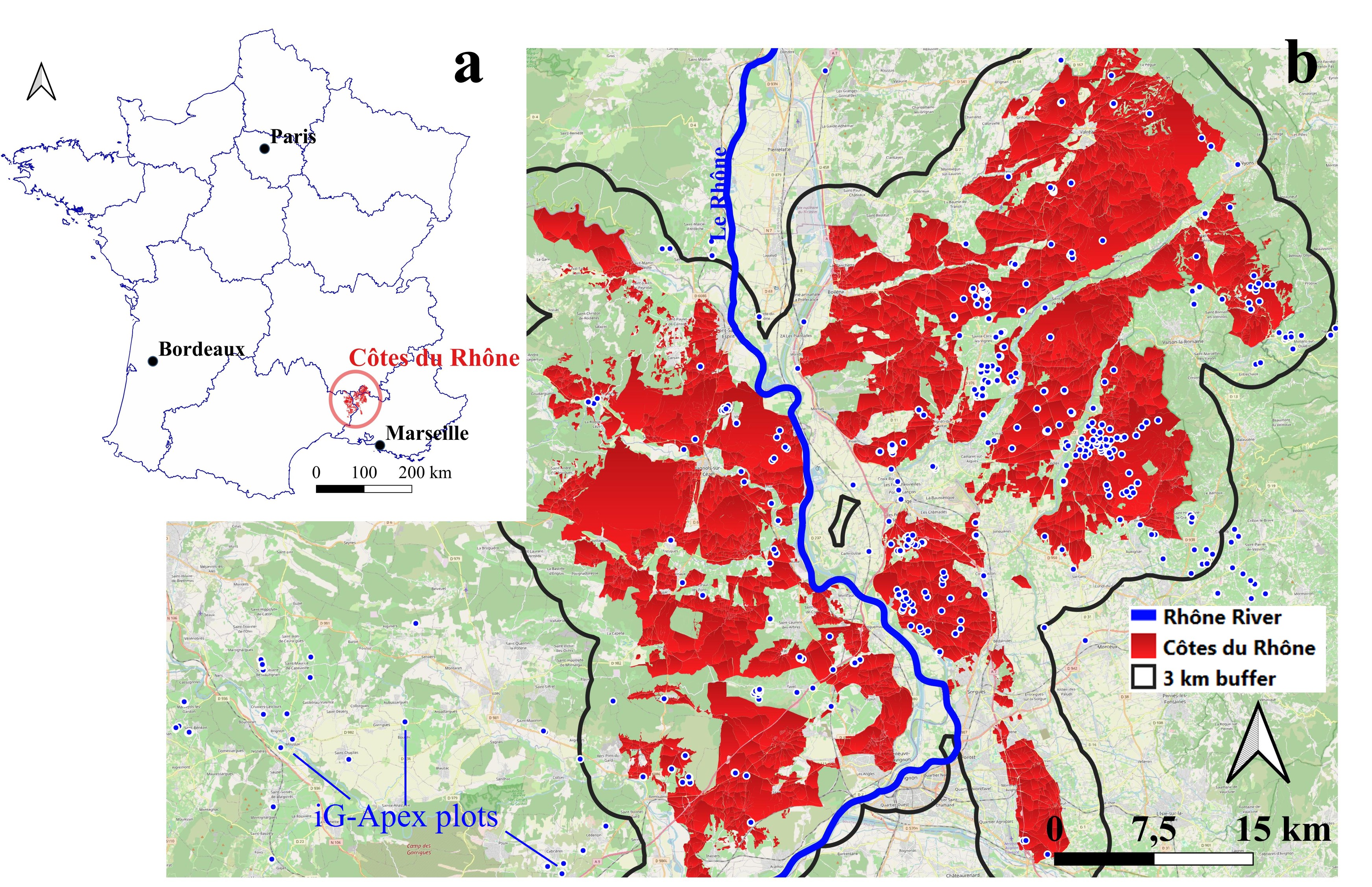
Figure 3. The study area, Côtes du Rhône (CDR): (a) location of CDR in France, (b) a zoomed view of the region with a 3 km buffer indicating crowdsourced data (blue dots) extraction zones.
A total of 2941 iG-Apex measurements (1749 TS) were collected over the study zone, with 227, 436, 408, 941, and 929 data points, respectively, in each year from 2019 to 2023. These measurements were selected from a 3 km buffer polygon created around the administrative boundaries of the CDR area (Figure 3b). A total of 25 weather cells (8 × 8 km) were contained in the zone.
4.2. Climatic conditions
The CDR is mainly dominated by a Mediterranean climate (Joly et al., 2010), characterised by warm temperate weather with hot dry summers (Köppen−Geiger climate type: Csa; Kottek et al., 2006). The Climatic Water Balance index (CWB = Daily precipitation – ET0) (Bandoc & Prăvălie, 2015) revealed a consistent summer water deficit across all five studied years. From 2019 to 2023, the annual CWB calculated between April and August was, respectively, –700 mm, –630 mm, –543 mm, –828 mm, and –607 mm. In terms of mean temperatures during the same period, year 2021 had the lowest mean temperature of 19.3 °C, in contrast with year 2022, which had the highest (22.0 °C). The mean temperatures for the remaining years (2019, 2020, 2023) were, respectively, 20.1, 20.4, and 20.5 °C. The years 2021 and 2022 were two contrasting vintages, with the former being rainy and cool, and the latter being dry and hot.
5. Evaluation of the results through a focus group
5.1. A “simulation by scenario” workshop
At the regional scale, no ground truth TTSW measurement was available for crowdsourcing plots. Hence, the approach chosen in this study was to rely on expert knowledge for assessing qualitative estimates at a large spatial scale, an approach that has been tested by Lopez-Fornieles et al. (2022).
Inspired by Pichon et al. (2019), the methodology was set up according to a “simulation by scenario” approach (Wacheux, 1996). In this approach, experts were invited to collectively build a TTSW map of the study area. They were invited to identify and rank distinct geographical zones according to three levels of TTSW: low, medium, and high. Experts first proposed an individual map on their own, then interacted with their peers to produce a collective map. This individual phase was set up so that each expert could express their opinions, even in the case of disagreement (Panebianco & Pahl-Wostl, 2004).
For the selection of experts, it was assumed that their knowledge of the CDR region, their experience in manipulating spatial information and their professional experience in viticulture could influence their estimation of different TTSW zones. Before the workshop, these three criteria were used to select experts who were as different as possible from each other (Table 1). It was decided to limit the number of experts to 5 to facilitate interaction between them.
Experts | ||||||
A | B | C | D | E | ||
Criteria | Knowledge of the CDR region | Intermediate | Intermediate | Advanced | Advanced | Intermediate |
Knowledge in spatial information | Advanced | Basic | Basic | Basic | Advanced | |
Professional experience in vines | Advanced | Advanced | Intermediate | Intermediate | Basic | |
The approach consisted of three main steps (Figure 4). In the first step (30 min), the experts were fully informed of the methodology applied in the focus group. In the second step (40 min), each expert was provided with a set of maps delineating different zones within the CDR. A total of 12 maps were distributed, corresponding to the following areas: “Northern Ardèche–Gard”, “Drôme Baronnies”, “Eastern Drôme”, “Northern Drôme”, “Southern Drôme”, “Rhodanian Gard”, “Southeastern Gard”, “Gigondas”, “Central Vaucluse and Dentelles de Vaucluse”, “Vaucluse Enclave and Southern Drôme”, “Rhodanian and Southern Vaucluse”, and the entire CDR region. On each map, vine plot locations were represented as unfilled polygons extracted from the French Land Parcel Identification System (LPIS; Registre Parcellaire Graphique, RPG). Using these materials, experts were asked to independently classify three levels of TTSW zones, using a predefined three-colour scheme. After this individual session, in the third step (30 min), the experts discussed their ranked zones and converged their own annotations onto a collective A0-format map. This map was then digitalised and used as the reference for evaluation.

Figure 4. Steps of focus group (workshop) with local experts and digitalisation; when expert A and B give respectively high and medium rank to the same zone, the medium rank is taken.
Situations where experts produced different TTSW ranks on the same geographical area could happen and were handled specifically: the lower rank was kept for presenting a pessimistic scenario, and the polygon was filled with a hatched pattern (Figure 4; e.g., when expert A and B give respectively high and medium rank to the same zone, then the medium rank is taken). The digitisation was carried out using QGIS 3.16.16-Hannover (QGIS Development Team, 2024).
5.2. Obtention of field and zonal estimation of TTSW
Due to the nature of crowdsourcing, it is possible that iG-Apex plots were highly clustered in space (Zhang & Zhu, 2018), while spatial clusters could not efficiently reflect the TTSW variability at the regional scale. Therefore, aggregated values of clustered estimates were obtained at the field level. Field averages were computed from individual estimates inside a field when the latter contains multiple estimates (Figure 5). Following the method presented by Taylor (1997), the average was inversely weighted by the uncertainty magnitude of TTSW estimates.
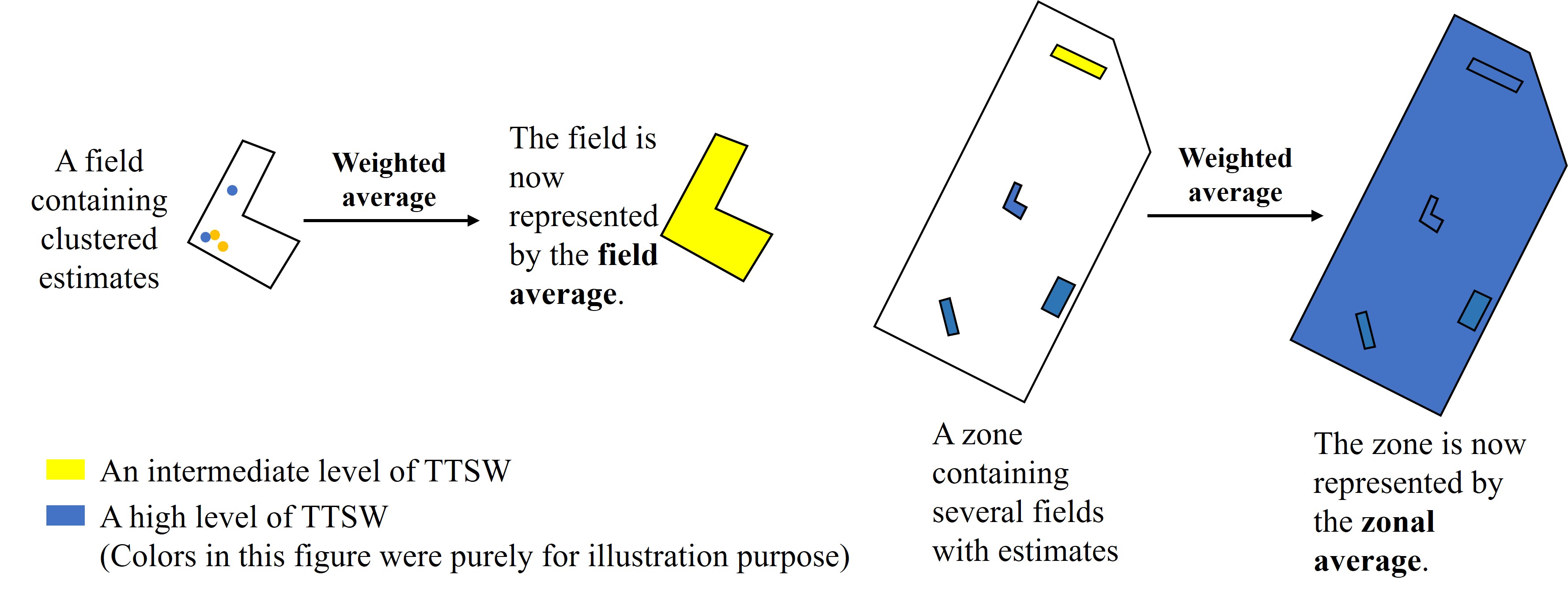
Figure 5. Steps for the obtention of field and zonal averages of TTSW (the colours in this figure were purely defined for illustration purposes).
Four confidence classes were established based on expert agreement and inversion results. Class A (high confidence) required both expert agreement (Section 5.1) and at least four field averages located inside an expert-defined polygon. Class B (moderate confidence) satisfied at least one of these criteria. Class C (low confidence) satisfied neither. Class D (not accessible) contained expert-defined polygons devoid of field averages.
During the evaluation phase after the workshop, experts defined geographical zones, each spanning several square kilometres, to represent areas with locally homogeneous TTSW. Each of these zones was a region that could contain multiple vine fields. Therefore, zonal averages could also be computed from field averages using the same method. This allows us to reveal a global level of TTSW inside a zone defined by experts for facilitating the evaluation.
Results
1. Pre-processed data and inverse model inputs
From 2019 to 2023, the Côte du Rhône (CDR) region exhibited variations in the timing of selected dry periods that satisfied the inverse model’s specific conditions (Figure 6a). The duration of these dry periods ranged from three weeks (in 2021) to nearly two months (in 2022). In 2021, the selected periods began notably late because of the occurrence of several rainfall events in June and July.
Based on the selected dry periods, the pre-processing retained 469 time series (TS) of iG-Apex out of the initial 1749 TS, which consisted of 859 iG-Apex measurements. A total of 449 retained TS were enriched, with nearly 380 TS being obtained after using both neighbouring data (spatial information) and simulated values (iG-Apex temporal information). These TS were dispersed in the region differently depending on vintages (Figure 6b). In 2021, there were the fewest retained TS (n = 1), because the majority of TS collected in that year were filtered out for not having enough observations inside selected dry periods. In contrast, year 2022 had TS homogeneously distributed and a rather high number of TS (n = 119). In year 2023, there were 180 TS (the highest number), although these TS were clustered in space (Figure 6.b presents a low number of visually identifiable points). In year 2019 and 2020, the numbers of retained TS were respectively 20 and 149.
The water status slope values of all retained TS ranged from –1.84*10–3 MPa/mm to –1.05*10–3 MPa/mm. Higher slope values indicated locations with potentially higher TTSW. In parallel, the average Kcb estimate was found to be 0.43, with a median of 0.45 and a standard deviation of 0.05. The minimum and maximum Kcb obtained in the CDR region were, respectively, 0.21 and 0.55. In addition, bootstrapping results revealed an average coefficient value of 0.47, with a median of 0.47 and a standard deviation of 0.03. Using the inverse model, these input values allowed us to obtain an estimated TTSW with associated uncertainty for each retained TS.
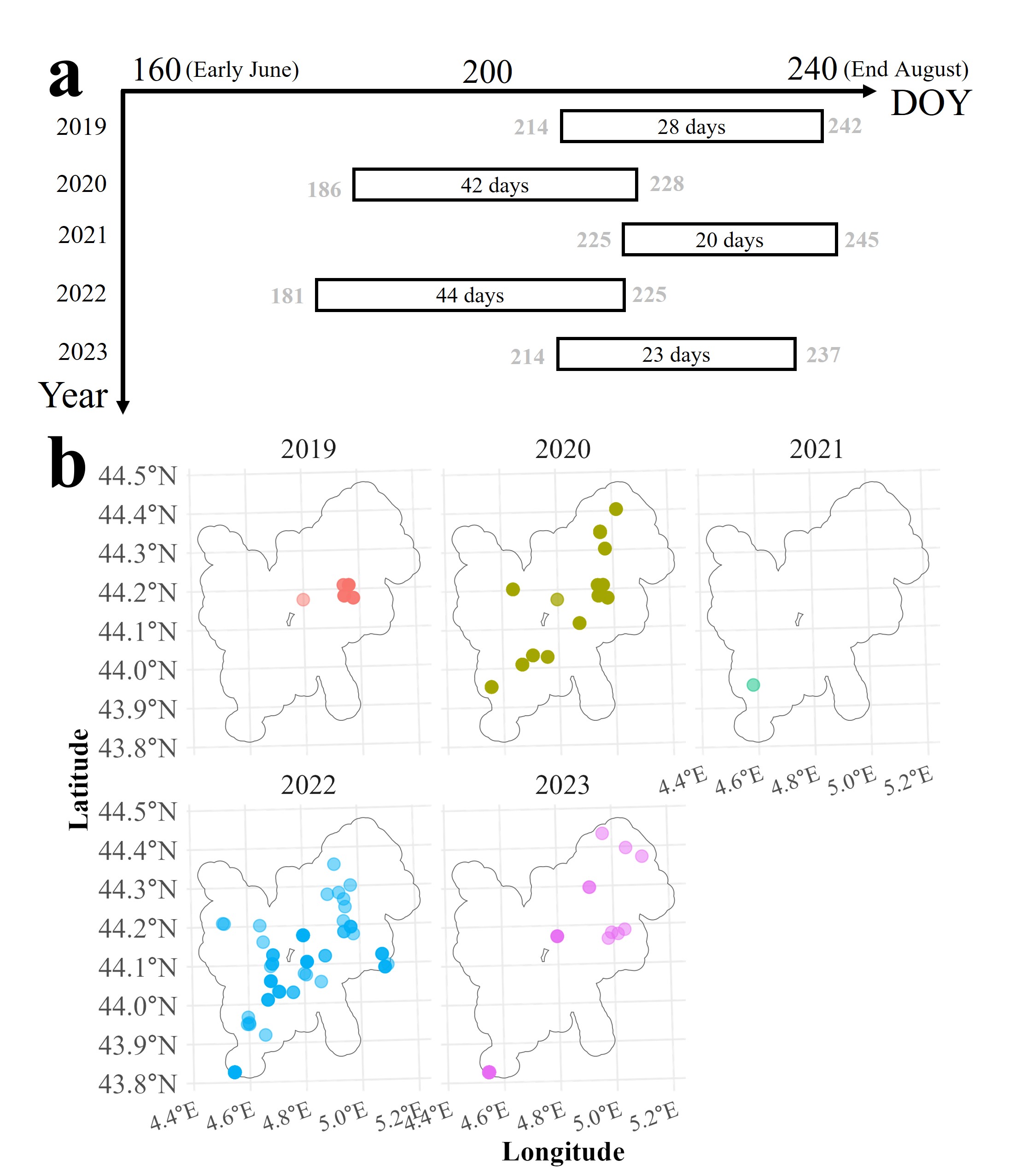
Figure 6. (a) Global positions (focusing on medians calculated from multiple locations in each year) of selected dry periods for inversion, and (b) spatial distribution of pre-processed iG-Apex plots in the Côte du Rhône (CDR) region.
2. Field averages of retrieved TTSW
The 469 retrieved TTSW values were contained inside 55 vine fields, allowing for the computation of 55 field averages. The average number of TTSW estimates contained in one field was 8. There were two exceptional fields that contained more than 30 TTSW estimates, including one field containing 202 values (indicating a highly clustered sampling behaviour).
The 55 field TTSW averages ranged from 60 mm to above 190 mm (Figure 7). The first quarter (0–25th percentile) of averages was lower than 100 mm, while the second quarter was below 112 mm. The third quarter was below 134 mm, in contrast to the last quarter, which exhibited a larger range of variability, spanning an interval of about 60 mm. In Figure 7, these quantiles were coloured to distinguish the three TTSW categories defined by the experts during the workshop, with the second and third quarters collapsed into a single class “Medium”.
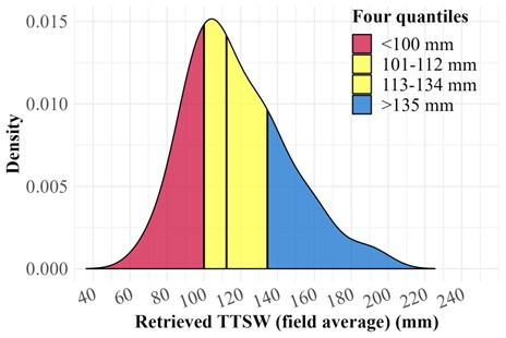
Figure 7. Density plot of the 55 field averages of retrieved TTSW coloured according to quantile intervals.
3. TTSW map generated by experts and comparison with retrieval results
Experts generated 27 polygons or groups of small polygons (numbered 1–27) within the CDR region during the focus group (Figure 8a). Each polygon represents a specific ranking class for TTSW. Experts disagreed on the classification of polygons 1, 2, 8, 12, 16, 20, and 25. One polygon in the western CDR was entirely excluded from classification due to high soil variability. Of the 55 total field TTSW values, 46 fell within the expert-defined boundaries (Figure 8b). Most polygons contained five or fewer field averages; specifically, polygons 4, 5, 21, and 26 contained only one. For each expert-generated polygon, a confidence class was attributed to (Table 2).
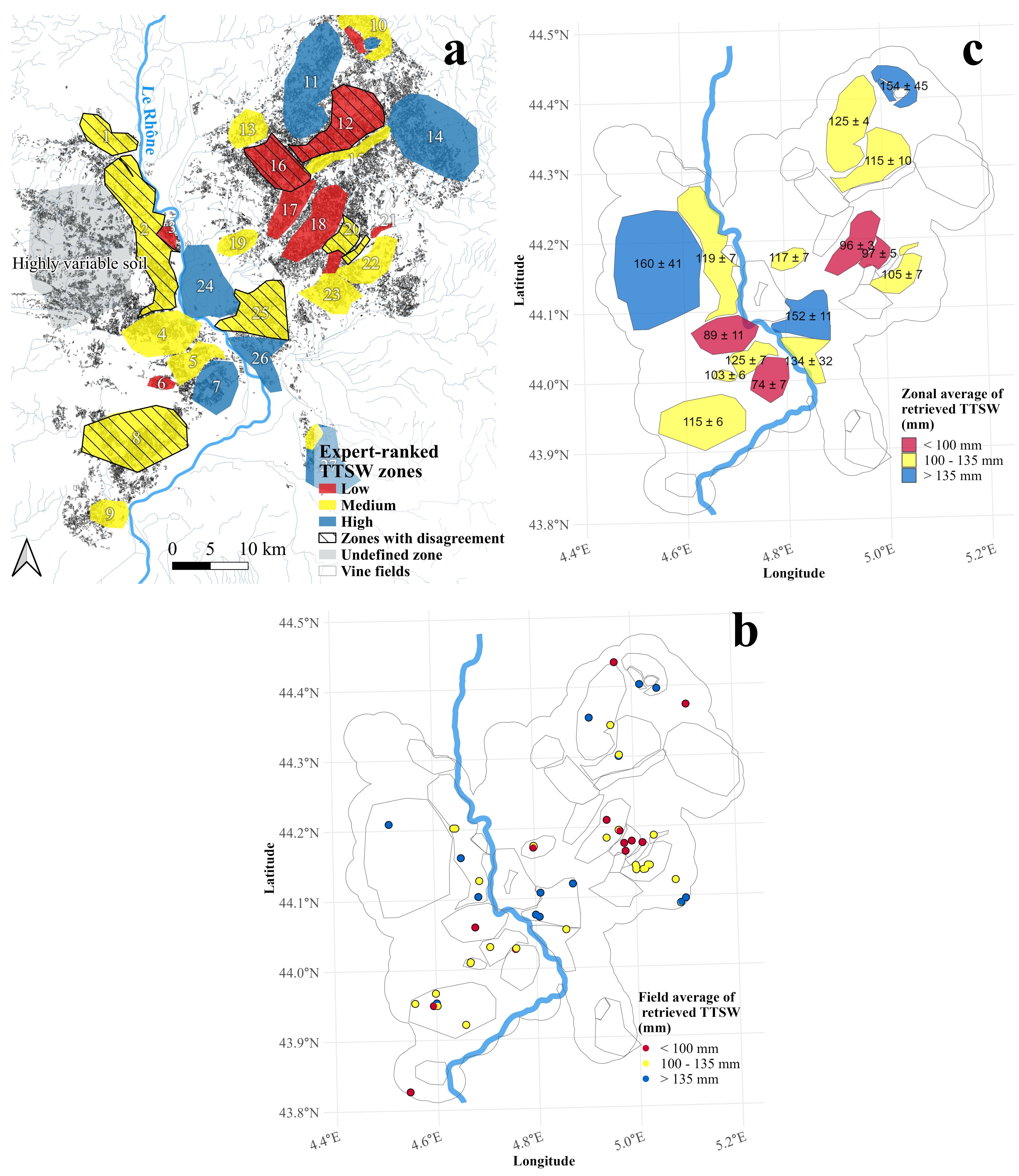
Figure 8. (a) Map of TTSW classes generated by experts, (b) Map of field averages of retrieved TTSW, and (c) Zonal averages of field TTSW values inside expert-defined zones in the CDR region. The three colours: red, yellow, and blue, corresponded to the 0–25 %, 25–75 %, and 75–100 % quantiles identified previously in Figure 7.
Confidence class | Involved polygons | Count |
A | 18, 22 | 2 |
B | 2, 4, 5, 6, 7, 8, 10, 11, 19, 20, 21, 25, 26 | 13 |
C | 12 | 1 |
D | 1, 3, 9, 13, 14, 15, 16, 17, 23, 24, 27 | 12 |
High-confidence polygons (18 and 22) demonstrated a clear alignment between expert rankings and calculated TTSW. Both areas are situated in the north-eastern CDR (Figure 8c). Similar agreements occurred in four intermediate-confidence polygons (2, 5, 8, and 19), where the TTSW rank was consistently medium. Three of these (2, 5, and 8) are located on the western bank of the Rhône River.
Other intermediate-confidence polygons also aligned with expert-defined classes. Polygon 6 (103 ± 6 mm) and polygon 20 (97 ± 5 mm) suggested low-to-medium TTSW (Figure 8c). Similarly, polygons 11, 25, and 26 yielded average values of 125, 152, and 134 mm, respectively. These values indicate a medium-to-high TTSW level, though they failed to achieve exact correspondence with expert classifications.
In contrast, several intermediate-confidence polygons showed significant discrepancies. Polygon 7 yielded a low TTSW estimate (74 ± 7 mm) despite being classified as "High" by experts. Polygon 4 (89 ± 11 mm) lacked coherence with the expert-defined "Medium" class. Polygon 10 similarly produced an incoherent result by overestimating the TTSW. Each of these misclassified polygons (4, 7, and 10) contained only one or two field averages.
Low-confidence polygons and those assigned to class D did not allow reliable interpretation, because the available validation data lacked sufficient robustness to support any conclusions.
Discussion
1. Coherence of retrieved values
This study retrieved TTSW at a regional scale using crowdsourced data and an inverse model for a Mediterranean wine-appellation: the Côtes du Rhône (CDR) in southeastern France. The field averages of retrieved TTSW showed a physically interpretable range of TTSW values that reflected realistic conditions in the viticultural lands of the CDR region (Coipel et al., 2006). For instance, in areas alongside the Rhône River, Fluviosols were highly prevalent, explaining the medium-to-high TTSW estimated from crowdsourcing data, while in the Eastern plain, soils were more calcareous and weathered, thereby being relatable to low-to-medium estimates (Messant et al., 2019). In contrast, under the soil erosion effect related to the Mediterranean climate, deep and structured soils are hard to form (e.g., Brown soils) in the study region, which partially explains why there were almost no TTSW values estimated beyond 200 mm.
Comparing with the expert-generated map, the spatial coherence of retrieved TTSW was particularly noticeable in two areas: one with medium-to-high TTSW ranking classes located along the Rhône River (polygons 2, 5, 8, 25, 26), and another with low-to-medium TTSW in the Eastern part of the region (polygons 18, 19, 20, 22) (Figure 8). These results might suggest that the approach can distinguish contrasting TTSW areas at a large spatial scale.
The expert-based evaluation method was designed to operate at the scale of the entire wine appellation. However, making quantitative evaluations with such data is challenging. Notably, it is difficult to provide a robust assessment of the confidence in experts’ opinions when this information was not explicitly elicited during the workshop. Although we distinguished three confidence levels by comparing the classes generated by experts—an a posteriori approach, a more a priori strategy could be implemented, for example by directly asking experts to report their confidence levels.
Additionally, comparing punctual TTSW estimations with the TTSW classes of expert-defined polygons is difficult due to their differing spatial footprints. Within an expert-defined polygon, the retrieved TTSW may locally deviate from the experts’ assessments because of local variability. This challenge was further compounded when only a few field averages were available within a polygon, which could explain the discrepancies observed in approximately 10 % of the studied cases, particularly in polygons 4, 7, 10, and 12. Future study should explore the minimum number of estimated TTSW for effectively representing not only a zonal value, but also the associated variance.
The results highlight the necessity to validate quantitatively TTSW estimates precisely at locations where observations were made, which was yet operationally difficult. The emergence of low-cost sensors (Vandôme et al., 2023) could reduce the difficulty of acquiring quantitative measurements. The framework of On Farm Experimentation (OFE) (Lacoste et al., 2022) might provide an opportunity to share reference values of TTSW: a survey should be conducted to identify locations with such data which allow for testing the inversion method on a large scale and based on field measurements of TTSW. Nonetheless, the qualitative evaluation method still permitted the identification of the incoherence of retrieved results, as four out of sixteen polygons contained contradictory results compared to the experts’ map. Various reasons could contribute to those errors, and they will be discussed hereafter.
2. Sources of error and implications
As an inverse model input, the water status slope coefficient could be incorrectly estimated. Applying a predictive model (i.e., the Recursive-Duo-Model (Zhang et al., 2024b)) over an entire region can be challenging, especially when considering that no training data were collected from such a spatial extent. Several factors could impact the predictive model’s performance negatively by altering the vine shoot growth itself. For instance, vine shoot growth, translated by the iG-Apex dynamic, could be dependent on the cultivar × rootstock pairs (Pichon et al., 2023). In the CDR region, although most vines were cv. Grenache, other cultivars such as cv. Syrah or cv. Cinsault also exist. Yet the cultivar and rootstock information were not accounted for. Furthermore, the row orientation and the density of vines in specific fields could generate competition for resources such as light, water and nutrients (Hunter et al., 2020), thereby affecting their vegetative growth. Similarly, vine shoot growth depends on soil management practices (e.g., tilling, intercropping), which also condition the vines access to resources (Zumkeller et al., 2023). Nevertheless, the relationship between these practices and iG-Apex is still unclear and was not considered. The deployed data-enrichment method, which assumes spatial and temporal autocorrelation in the observations, could also introduce additional error into the water-status slope, a limitation fundamentally related to the lack of high-quality data in crowdsourcing (see Discussion Section 4). It is possible that a TTSW estimated using a reconstructed TS is less reliable than one estimated using a complete TS. The uncertainty could be considered in a future study.
The estimated Kcb may represent another major source of error. Ground-truth Kcb data are lacking, and the predictive model derived from satellite imagery would be substantially improved from such observations. Moreover, although the IM approach assumes bare soil conditions to maximise simplification of vineyard systems, actual observation sites (e.g., iG-Apex) may retain inter-row cover crops, which can influence NDVI measurements and thereby introduce additional bias.
When applicable, a vine field might be irrigated in the studied region (Cambrea et al., 2020). If iG-Apex measurements were collected from an irrigated field, vine shoot growth might not accurately reflect the actual field TTSW. Yet, this information was not accessible. Another piece of missing information that could be a source of error could equally be the plot area ratio, which was set to be 0.85 for all plots, while it can vary significantly from one plot to another.
Such lack of information might imply some potential updates which could be integrated into the Apex-Vigne application. For instance, a simple confirmation on the presence of cover crops could be required. Concerning the plot area ratio, the APP could ask for the number of unproductive vines included in an observation plot. This count could then be used to obtain an estimation of the plot area ratio. Similarly, cultivar information could also be collected. The additional required input from users could, however, complicate data collection, which was discussed in the next section. In parallel, ancillary data sources could be deployed. For instance, it is possible to use Sentinel-2 satellite images to identify inter-row management practices (Devaux et al., 2019). This information could be used to adjust the Kcb estimated from NDVI. Additionally, weather data with a higher spatial resolution might improve the description of the climatic context related to Crowdsourcing plots, thereby improving the accuracy.
3. Potentials and limitations related to the crowdsourcing approach
The lack of information discussed previously might be a result of the trade-off between the ease of data collection and the amount of collected data (Li et al., 2021). Apex-Vigne required very little information from its users, in exchange for a considerable number of vine shoot growth observations. Within five years, the tool gathered almost 30,000 iG-Apex measurements. Considering that one single measurement takes five minutes, the total equivalent amount of fieldwork hours was significant (2500 hours). Additionally, most data collectors were unaware of the possibility to transform observations they made into TTSW: highly valuable information not only for regional structures, but also for growers themselves. Therefore, the motivation of collecting iG-Apex data might further be incited if data collectors became more aware of the scientific perspective of the project.
Nevertheless, currently, less than 30 % of collected time series were used in inversion. Indeed, most time series were removed during the pre-processing phase, because many of them contained fewer than three observations, which limited the ability to obtain the sigmoid curve describing the iG-Apex dynamic and, consequently, the enrichment algorithm.
In parallel, the filtered dataset was spatially heterogeneous. The number of field averages in high TTSW areas defined by experts was merely 5, which was largely inferior to the two other types of area (10 in low TTSW, 31 in medium TTSW). However, it might make sense that data collectors focused more on monitoring fields with a potentially higher risk of drought (low to medium TTSW), instead of monitoring vines with a low risk (high TTSW). This motivation might explain the presence of low TTSW values (corresponding to sites where the risk of drought is high) in zones where experts indicated a high TTSW level. Evidence of such a “risk-oriented” sampling strategy could be found by comparing data collected from different vintages. In 2022, the driest vintage, crowdsourcing took place in a more global manner inside the CDR region, in contrast with other vintages (Figure 6b; with special focus on year 2021, which is the least dry among five years).
Assessing the interannual variability of estimated TTSW using crowdsourced data is challenging, as such an analysis requires repeated measurements at the same locations, ideally on the same plants, over multiple years with contrasting climatic conditions and under controlled observational protocols. In contrast, crowdsourced data are collected at arbitrary locations, which limits their suitability for longitudinal analysis. Dedicated research efforts are therefore needed to evaluate the temporal stability of the inversion method.
4. Suggestions to improve TTSW retrieved from crowdsourced data
To increase the ratio of iG-Apex data deployable for TTSW retrieval, data collectors should be encouraged to gather long time series (at least 4 per plot per season) that contain at least four observations at fewer locations, rather than collecting abundant single measurements or very short series at many different locations.
However, generating a longer time series requires spanning weekly measurements at least over a month, which may negatively impact data collectors’ motivation (Rotman et al., 2012). To address this challenge, future research should focus on identifying pivot points that incentivise data collectors to repeat the same task at the same location. One potential solution is to effectively communicate the practical benefits that data collectors could gain from their contributions, which may enhance their beliefs about the causal impact of their efforts (Goncalves et al., 2015). For example, scenarios where estimated TTSW assists in decision-making processes could be communicated to APP users, such as showing the meaning of knowing TTSW for different farming practices (Chandler & Kapelner, 2013). Additionally, promoting an Apex-Vigne user community (Kosonen et al., 2013) where observations, analyses, and thoughts related to vine shoot growth could be easily shared might also incentivise data collectors' motivation and facilitate practice shifting.
Reducing the spatial heterogeneity of data requires the application of a more homogeneous sampling strategy. However, this is inherently challenging due to the opportunistic nature of crowdsourcing projects (De Vos et al., 2023). Additionally, most Apex-Vigne users are professionals whose main motivation for data collection is egoistic and extrinsic (i.e., they try to perform a task related to their professional activity), rather than altruistic or collective (i.e., they voluntarily want to help researchers, or to contribute to the common good) (Pichon, 2021). These obstacles must be properly addressed by future research. The On Farm Experiment (OFE) framework might be a promising solution, as it explicitly acknowledges the private interests of farmers and other OFE participants (Lacoste et al., 2022). This framework may create an appropriate situation where the effort of applying a more organised sampling strategy could be traded with the gain of knowledge on spatial TTSW variation.
Conclusion
This study presents an inverse modelling approach that integrates crowdsourced data to retrieve grapevine Total Transpirable Soil Water (TTSW) at a regional scale. Retrieved values ranged from 60 to 190 mm, a result physically consistent with the region’s predominant soil types. This inversion approach was evaluated through a qualitative comparison with a TTSW map generated by local experts.
High-confidence areas, where expert opinions converged and at least four field averages existed, demonstrated coherent TTSW rankings. While most intermediate-confidence areas showed similar alignment, some specific zones performed poorly. Collectively, these results identified two distinct geographical regions: one characterised by low-to-medium TTSW and another by medium-to-high levels. This spatial differentiation suggests that crowdsourced data, when combined with inverse modelling, can effectively reveal broad-scale TTSW patterns.
However, certain limitations remain. Inaccurate estimates persisted in some polygons, and the inverse model used less than 30 % of the total crowdsourced observations. This low utilisation rate occurred because most collected time series were either too short or too spatially isolated for effective inversion.
Future research should focus on identifying incentives that encourage data collectors to maintain longer time series. Efforts should also promote the integration of scientifically robust sampling strategies. Finally, researchers should validate this approach using quantitative reference data across contrasting environmental settings to maximise the potential of regional-scale TTSW monitoring.
Acknowledgements
This work was supported by the French National Research Agency under the Investments for the Future Program, referred to as ANR-16-CONV-0004. The Apex-Vigne project was part of the DATI project, supported by the French National Research Agency under the Horizon 2020 PRIMA Program (ANR-21-PRIM-0001). The authors would like to thank J-C. Payan for his invaluable help.
References
- Acevedo-Opazo, C., Tisseyre, B., Guillaume, S., & Ojeda, H. (2008). The potential of high spatial resolution information to define within-vineyard zones related to vine water status. Precision Agriculture, 9(5), 285–302. https://doi.org/10.1007/s11119-008-9073-1
- Alkassem, M., Buis, S., Coulouma, G., Jacob, F., Lagacherie, P., & Prévot, L. (2022). Estimating soil available water capacity within a Mediterranean vineyard watershed using satellite imagery and crop model inversion. Geoderma, 425, 116081. https://doi.org/10.1016/j.geoderma.2022.116081
- Bandoc, G., & Prăvălie, R. (2015). Climatic water balance dynamics over the last five decades in Romania’s most arid region, Dobrogea. Journal of Geographical Sciences, 25(11), 1307–1327. https://doi.org/10.1007/s11442-015-1236-1
- Bertuzzi, P., & Clastre, P. (2022). Information sur les mailles SAFRAN (Version 1). Recherche Data Gouv. https://doi.org/10.57745/1PDFNL
- Brillante, L., Mathieu, O., Bois, B., van Leeuwen, C., & Lévêque, J. (2015). The use of soil electrical resistivity to monitor plant and soil water relationships in vineyards. SOIL, 1(1), 273–286. https://doi.org/10.5194/soil-1-273-2015
- Brunel, G., Pichon, L., Taylor, J., & Tisseyre, B. (2019). Easy water stress detection system for vineyard irrigation management. In Precision agriculture 2019 (pp. 935–942). Wageningen Academic Publishers. https://doi.org/10.3920/978-90-8686-888-9_115
- Cambrea, L., Lafon, C., & Mayoux, L. (2020). Live from the regions – Vine irrigation in the former Languedoc-Roussillon region: Production potential maintained through water savings. Sciences Eaux & Territoires, 34bis, Article 34bis. https://doi.org/10.14758/SET-REVUE.2020.4.05
- Campos, I., Neale, C. M. U., Calera, A., Balbontín, C., & González-Piqueras, J. (2010). Assessing satellite-based basal crop coefficients for irrigated grapes (Vitis vinifera L.). Agricultural Water Management, 98(1), 45–54. https://doi.org/10.1016/j.agwat.2010.07.011
- Celette, F., Ripoche, A., & Gary, C. (2010). WaLIS—A simple model to simulate water partitioning in a crop association: The example of an intercropped vineyard. Agricultural Water Management, 97(11), 1749–1759. https://doi.org/10.1016/j.agwat.2010.06.008
- Chandler, D., & Kapelner, A. (2013). Breaking monotony with meaning: Motivation in crowdsourcing markets. Journal of Economic Behavior & Organization, 90, 123–133. https://doi.org/10.1016/j.jebo.2013.03.003
- Coipel, J., Lovelle, B. R., Sipp, C., & Leeuwen, C. van. (2006). ‘Terroir’ effect, as a result of enviromental stess, depends more on soil depth than on soil type (Vitis vinifera) L. cv. Grenache Noir, Côtes du Rhône, France, 2000). OENO One, 40(4), Article 4. https://doi.org/10.20870/oeno-one.2006.40.4.867
- Coppola, A., Dragonetti, G., Comegna, A., Lamaddalena, N., Caushi, B., Haikal, M. A., & Basile, A. (2013). Measuring and modeling water content in stony soils. Soil and Tillage Research, 128, 9–22. https://doi.org/10.1016/j.still.2012.10.006
- Coulouma, G., Prevot, L., & Lagacherie, P. (2020). Carbon isotope discrimination as a surrogate for soil available water capacity in rainfed areas: A study in the Languedoc vineyard plain. Geoderma, 362, 114121. https://doi.org/10.1016/j.geoderma.2019.114121
- Cousin, I., Buis, S., Lagacherie, P., Doussan, C., Le Bas, C., & Guérif, M. (2022). Available water capacity from a multidisciplinary and multiscale viewpoint. A review. Agronomy for Sustainable Development, 42(3), 46. https://doi.org/10.1007/s13593-022-00774-8
- Devaux, N., Crestey, T., Leroux, C., & Tisseyre, B. (2019). Potential of Sentinel-2 satellite images to monitor vine fields grown at a territorial scale. OENO One, 53(1), Article 1. https://doi.org/10.20870/oeno-one.2019.53.1.2293
- De Vos, K., Campforts, B., Tits, L., Van Tricht, K., Bonte, K., Govers, G., & Jacobs, L. (2023). Potential and limitations of crowdsourced data for high-resolution rice mapping in Madagascar: The importance of representation. International Journal of Applied Earth Observation and Geoinformation, 117, 103204. https://doi.org/10.1016/j.jag.2023.103204
- Fernandez-Mena, H., Guilpart, N., Lagacherie, P., Roux, R. L., Plaige, M., Dumont, M., Gautier, M., Graveline, N., Touzard, J.-M., Hannin, H., & Gary, C. (2023). Grapevine yield gap: Identification of environmental limitations by soil and climate zoning in the region of Languedoc-Roussillon (South of France). OENO One, 57(2), Article 2. https://doi.org/10.20870/oeno-one.2023.57.2.7246
- Gaudin, R., Roux, S., & Tisseyre, B. (2017). Linking the transpirable soil water content of a vineyard to predawn leaf water potential measurements. Agricultural Water Management, 182, 13–23. https://doi.org/10.1016/j.agwat.2016.12.006
- Goncalves, J., Hosio, S., Rogstadius, J., Karapanos, E., & Kostakos, V. (2015). Motivating participation and improving quality of contribution in ubiquitous crowdsourcing. Computer Networks, 90, 34–48. https://doi.org/10.1016/j.comnet.2015.07.002
- Hunter, J. K., Tarricone, L., Volschenk, C., Giacalone, C., Melo, M. S., & Zorer, R. (2020). Grapevine physiological response to row orientation-induced spatial radiation and microclimate changes. OENO One, 54(2), Article 2. https://doi.org/10.20870/oeno-one.2020.54.2.3100
- INAO. (2024). AOC Côtes du Rhône (https://www.inao.gouv.fr/show_texte/834). INAO. https://www.inao.gouv.fr/show_texte/834
- Joly, D., Brossard, T., Cardot, H., Cavailhes, J., Hilal, M., & Wavresky, P. (2010). Les types de climats en France, une construction spatiale. Cybergeo: European Journal of Geography. https://doi.org/10.4000/cybergeo.23155
- Kosonen, M., Gan, C., Olander, H., & Blomqvist, K. (2013). My idea is our idea! Supporting user-driven innovation activities in crowdsourcing communities. International Journal of Innovation Management, 17(03), 1340010. https://doi.org/10.1142/S1363919613400100
- Kottek, M., Grieser, J., Beck, C., Rudolf, B., & Rubel, F. (2006). World Map of the Köppen-Geiger climate classification updated. Meteorologische Zeitschrift, 259–263. https://doi.org/10.1127/0941-2948/2006/0130
- Lacoste, M., Cook, S., McNee, M., Gale, D., Ingram, J., Bellon-Maurel, V., MacMillan, T., Sylvester-Bradley, R., Kindred, D., Bramley, R., Tremblay, N., Longchamps, L., Thompson, L., Ruiz, J., García, F. O., Maxwell, B., Griffin, T., Oberthür, T., Huyghe, C., … Hall, A. (2022). On-Farm Experimentation to transform global agriculture. Nature Food, 3(1), 11–18. https://doi.org/10.1038/s43016-021-00424-4
- Lakso, A., & Eissenstat, D. (2012). Fifteen Years of Vine Root Growth Studies in Concords (https://www.semanticscholar.org/paper/Fifteen-Years-of-Vine-Root-Growth-Studies-in-Lakso-Eissenstat/325f612c0e4c5100ca4c2ffdb9e4305c0728bf34 ).
- Lebon, E., Dumas, V., Pieri, P., & Schultz, H. R. (2003). Modelling the seasonal dynamics of the soil water balance of vineyards. Functional Plant Biology, 30(6), 699–710. https://doi.org/10.1071/fp02222
- Lebon, E., Pellegrino, A., Louarn, G., & Lecoeur, J. (2006). Branch Development Controls Leaf Area Dynamics in Grapevine (Vitis vinifera) Growing in Drying Soil. Annals of Botany, 98(1), 175–185. https://doi.org/10.1093/aob/mcl085
- Leenaars, J. G. B., Claessens, L., Heuvelink, G. B. M., Hengl, T., Ruiperez González, M., van Bussel, L. G. J., Guilpart, N., Yang, H., & Cassman, K. G. (2018). Mapping rootable depth and root zone plant-available water holding capacity of the soil of sub-Saharan Africa. Geoderma, 324, 18–36. https://doi.org/10.1016/j.geoderma.2018.02.046
- Li, Y., Chang, L., Li, L., Bao, X., & Gu, T. (2021). Key Research Issues and Related Technologies in Crowdsourcing Data Collection. Wireless Communications and Mobile Computing, 2021(1), 8745897. https://doi.org/10.1155/2021/8745897
- Lopez-Fornieles, E., Brunel, G., Devaux, N., Roger, J.-M., Taylor, J., & Tisseyre, B. (2022). Application of Parallel Factor Analysis (PARAFAC) to the Regional Characterisation of Vineyard Blocks Using Remote Sensing Time Series. Agronomy, 12(10), Article 10. https://doi.org/10.3390/agronomy12102544
- Menn, N. L., Leeuwen, C. van, Riquier, L., Revel, G. de, & Marchand, S. (2020). How can the water regime and nitrogen status of the vine influence aging aromas in red wines? Original language of the article: French. IVES Technical Reviews, Vine and Wine. https://doi.org/10.20870/IVES-TR.2020.3984
- Messant, A., Chafchafi, A., Ducommun, C., Jalabert, S., Lagacherie, P., Lehmann, S., Lemercier, B., Moulin, J., Mure, J.-P., Noraz, A., Laroche, B., & Sauter, J. (2019). Les sols dominants en France métropolitaine. 46 p. (https://hal.inrae.fr/hal-04315558 ).
- Panebianco, S., & Pahl-Wostl, C. (2004). Obstacles in Launching a Participatory Group Discussion and Modelling Process. International Congress on Environmental Modelling and Software. https://scholarsarchive.byu.edu/iemssconference/2004/all/118
- Pellegrino, A., Lebon, E., Voltz, M., & Wery, J. (2005). Relationships between plant and soil water status in vine (Vitis vinifera L.). Plant and Soil, 266(1), 129–142. https://doi.org/10.1007/s11104-005-0874-y
- Pichon, L. (2021). Development of a crowdsourcing approach adapted to agriculture specificities: The case of monitoring vine water status with the shoot growth approach [Phdthesis, Montpellier SupAgro]. https://theses.hal.science/tel-04065976
- Pichon, L., Brunel, G., Zhang, Y., & Tisseyre, B. (2022). Towards a regional mapping of vine water status based on crowdsourcing observations: This article is published in cooperation with Terclim 2022 (XIVth International Terroir Congress and 2nd ClimWine Symposium), 3-8 July 2022, Bordeaux, France. OENO One, 56(2), Article 2. https://doi.org/10.20870/oeno-one.2022.56.2.5442
- Pichon, L., Laurent, C., Payan, J.-C., & Tisseyre, B. (2023). Observation of shoot growth: A simple and operational decision-making tool for monitoring vine water status in the vineyard. OENO One, 57(1), Article 1. https://doi.org/10.20870/oeno-one.2023.57.1.5481
- Pichon, L., Leroux, C., Macombe, C., Taylor, J., & Tisseyre, B. (2019). What relevant information can be identified by experts on unmanned aerial vehicles’ visible images for precision viticulture? Precision Agriculture, 20(2), 278–294. https://doi.org/10.1007/s11119-019-09634-0
- QGIS Development Team, 2024. (n.d.). Retrieved 23 April 2024, from https://issues.qgis.org/projects/qgis/wiki/QGIS_Citation_Repository
- Rallo, G., Paço, T. A., Paredes, P., Puig-Sirera, À., Massai, R., Provenzano, G., & Pereira, L. S. (2021). Updated single and dual crop coefficients for tree and vine fruit crops. Agricultural Water Management, 250, 106645. https://doi.org/10.1016/j.agwat.2020.106645
- R Core Team. (2021). R: A Language and Environment for Statistical Computing [Computer software]. R Foundation for Statistical Computing. https://www.R-project.org/
- Rotman, D., Preece, J., Hammock, J., Procita, K., Hansen, D., Parr, C., Lewis, D., & Jacobs, D. (2012). Dynamic changes in motivation in collaborative citizen-science projects. Proceedings of the ACM 2012 Conference on Computer Supported Cooperative Work, 217–226. https://doi.org/10.1145/2145204.2145238
- Santillán, D., Iglesias, A., La Jeunesse, I., Garrote, L., & Sotes, V. (2019). Vineyards in transition: A global assessment of the adaptation needs of grape producing regions under climate change. Science of The Total Environment, 657, 839–852. https://doi.org/10.1016/j.scitotenv.2018.12.079
- Surowiecki, J. (2004). The wisdom of crowds: Why the many are smarter than the few and how collective wisdom shapes business, economies, societies, and nations (pp. xxi, 296). Doubleday & Co.
- Taylor, J. R. (1997). An Introduction to Error Analysis: The Study of Uncertainties in Physical Measurements (2nd Edition). University Science Books.
- Ucar, I., & Henry, L. (2023). errors: Uncertainty Propagation for R Vectors (Version 0.4.1) [Computer software]. https://cran.r-project.org/web/packages/errors/index.html
- Vandôme, P., Leauthaud, C., Moinard, S., Sainlez, O., Mekki, I., Zairi, A., & Belaud, G. (2023). Smart agricultural technology. Smart Agricultural Technology, 4, Article 100227. https://doi.org/10.1016/j.atech.2023.100227
- van Leeuwen, C., Roby, J.-P., & Rességuier, L. de. (2018). Soil-related terroir factors: A review. OENO One, 52(2), Article 2. https://doi.org/10.20870/oeno-one.2018.52.2.2208
- Vaudour, E., Girard, M.-C., Bremond, L.-M., & Lurton, L. (1998). Spatial terroir characterization and grape composition in the Southern Côtes-du-Rhône vineyard (Nyons-Valreas Basin). OENO One, 32(4), Article 4. https://doi.org/10.20870/oeno-one.1998.32.4.1043
- Vaudour, E., Leclercq, L., Gilliot, J. M., & Chaignon, B. (2017). Retrospective 70 y-spatial analysis of repeated vine mortality patterns using ancient aerial time series, Pléiades images and multi-source spatial and field data. International Journal of Applied Earth Observation and Geoinformation, 58, 234–248. https://doi.org/10.1016/j.jag.2017.02.015
- Wacheux, F. (1996). Méthodes qualitatives de recherches en gestion. Economia. https://hal.science/hal-00157140
- Zhang, G., & Zhu, A.-X. (2018). The representativeness and spatial bias of volunteered geographic information: A review. Annals of GIS, 24(3), 151–162. https://doi.org/10.1080/19475683.2018.1501607
- Zhang, Y., Pichon, L., Pellegrino, A., Roux, S., Péruzzaro, C., & Tisseyre, B. (2024b). Predicting predawn leaf water potential while accounting for uncertainty using vine shoot growth and weather data in Mediterranean rainfed vineyards. Agricultural Water Management, 302, 108998. https://doi.org/10.1016/j.agwat.2024.108998
- Zhang, Y., Pichon, L., Roux, S., Pellegrino, A., Coulouma, G., & Tisseyre, B. (2025). Retrieving total transpirable soil water in a rainfed vineyard using vine shoot growth, weather, and Sentinel-2 data. Agricultural Water Management, 318, 109760. https://doi.org/10.1016/j.agwat.2025.109760
- Zhang, Y., Pichon, L., Roux, S., Pellegrino, A., Simonneau, T., & Tisseyre, B. (2024a). Why make inverse modeling and which methods to use in agriculture? A review. Computers and Electronics in Agriculture, 217, 108624. https://doi.org/10.1016/j.compag.2024.108624
- Zumkeller, M., Torres, N., Yu, R., Marigliano, L. E., Zaccaria, D., Tanner, J. D., & Kurtural, S. K. (2023). Cover crops and no-tillage show negligible effects on grapevine physiology in mediterranean vineyard agroecosystems. OENO One, 57(2), Article 2. https://doi.org/10.20870/oeno-one.2023.57.2.7136
 Views: 388
 XML: 59